- Research
- Open access
- Published:
Influential spatial facility prediction over large scale cyber-physical vehicles in smart city
EURASIP Journal on Wireless Communications and Networking volume 2016, Article number: 103 (2016)
Abstract
Facilities are critical infrastructures in smart city. Influence of facilities is affected by large-scale moving objects such as people and vehicles. Calculating the influence of facilities is an important task of urban computing, which adopts sensing technology to obtain objects’ movement patterns in urban space and applies this information to discover many hidden issues cities face today. In this paper, we propose a computationally efficient grid partition method to compute the influence of facilities in real time, under trajectories of large-scale cyber-physical vehicles. We next predict the influence changes of facilities over dynamic vehicles using trajectory-based Markov model. We conduct evaluation using a real-world dataset, including 1-month taxi trajectories with 27,000 taxis and 1000 facilities. Experimental results shows that our solution is more efficient and achieves an accuracy of 85 %.
1 Introduction
Cyber-physical vehicles [1, 2] have emerged to focus on the integration of sensing, computing, and actuation technologies into everyday urban settings and lifestyles. In cyber-physical vehicle system, locations of vehicles are the key information which not only interact dynamics of connected vehicles but also provide people a new perspective to modern city [3–5]. Understanding the influences of dynamic vehicles may help urban planners to make more informed decisions. For instance, urban planners can use massive GPS location data from taxis to help analyzing traffic anomalies [6], area functions [7], travel routes [8], etc.
Nowadays, modern urban has a variety of public infrastructures including subway stations, overpasses, office facilities, sports arenas, supermarkets, convention centers, hospitals, and entertainment parks, to name a few. They support different needs of people’s urban lives and serve as a valuable tool for getting a detailed understanding of how a metropolitan area works. These infrastructures are called facilities [9–11], which aim to provide location-dependent services in smart city.
To monitor the service behavior of facilities, various sensor networks have been deployed in facilities. Previous sensor-based works mainly focused on coverage [12], routing [13, 14], data aggregation [15, 16], and sensory data analytics [17]. However, moving people and vehicles outside facilities also need to be monitored and analyzed. On the one hand, facilities have varying degrees of influence that heavily affects people’s lifestyle. On the other hand, vehicles can generate time-varying and dynamic influence to nearby facilities. For instance, overpasses have different influences over vehicles in different times. An overpass in downtown is crowded by vehicles during rush hours on weekdays than in the suburb. In the evening, however, there are more vehicles close to overpasses in the suburb than in the downtown area. As we see from the example, dynamic mobility of vehicles significantly affects the influence of facilities. What the urban administrator cares about is what’s the most influential facilities [11, 18] now and in the future. In this paper, we compute and predict the influence of facilities by considering massive dynamic moving vehicles.
While the idea of using the count of moving vehicles to compute and predict the influence of facilities seems simple, several challenges arise in practice. The first challenge is how to efficiently calculate the influence of facilities given massive vehicles and facilities. Urban real-time monitoring system requires facility influence to be updated as far as possible. Naive counting method and R-tree index [11] in geodatabase suffer from too much computing overhead. The second challenge is how to predict future influence of facilities when only current locations of vehicles are known. The number of vehicles around a facility at this moment cannot be used to compute the influence in the future. This is because vehicles move around and this dynamic movements leads to varying influence of facilities over time.
In this paper, we propose our ideas to address these two challenges based on the following intuitions. Firstly, some time-consuming operations such as traversing and distance computing can be replaced by lightweight mapping functions approximately. We use a grid index method which maps a vehicle location to a specific cell, and the count of vehicles within this cell is added to the influence of its nearest facility. Another intuition is that, every vehicle has its own trajectory and if two vehicles have similar trajectories, they will go to the same area in next time unit with a high probability. In particular, we use trajectory-based Markov chain model (TMM), a variation of Markov chain learned by historical movements, to predict new vehicles’ movements and then update future facility influence.
We validate our solution using a large real-world dataset which consists of 1-month moving trajectories of taxis in Beijing. Facilities of interest are subway stations, overpasses, and shopping malls extracted from point of interests (POIs) in Beijing. Experimental results show that our solutions are effective and efficient in computing and in predicting facility influence under large-scale cyber-physical vehicles.
The rest of the paper is organized as follows. Section 2 presents the problem of facility influence calculation. We then propose a grid partition approach to efficiently compute facility influence in Section 3. Trajectory-based Markov model is designed to predict vehicle’s location in the future (Section 4). In Section 5, we evaluate our solution using a large-scale dataset. Finally, we introduce related work and make concluding remarks.
2 Problem definition
In this section, we discuss the definition of facility influence over moving objects such as vehicles and propose two problems.
Influential facility computing was first introduced in [11] where the influence of facility f is defined as the number of objects that consider f as the nearest site among all objects. A modern city has many facilities such as supermarkets, subway stations, and entertainment parks. These facilities provide a variety of services to people and cars. As a result, peoples or vehicles often gather around these facilities. When and how they go to a particular facility are determined by many factors including the services provided, the quality of the facility, and people’s lifestyle and so on. No matter why objects go to different facilities, more objects means the larger influence the facility has. Figure 1 shows three facilities {f 1, f 2, f 3} having 3, 2, and 1 vehicle(s), respectively. In this case, f 1 has the highest influence.

Facility influence. Black dots are facilities and white circles are vehicles
In general, moving objects include but are not limited to vehicles and people. The proposed algorithms in this paper can also be used for facilities and other moving objects. In the following sections, we do not differentiate terms “vehicle,” “object,” and “moving object”. Let \(\mathcal {P}\) denote a set of objects and \(\mathcal {F}\) a set of facilities. Assume object \(p \in \mathcal {P}\) and facility \(f \in \mathcal {F}\). We denote the influence of facility f as
Definition 1 (Facility Influence).
For every facility f, the influence of f is defined as the total number of objects in its influence range at specific time stamp.
where R f (p) is a Boolean function: it equals 1 if object p appears in the range of the facility f, otherwise equals 0. Function R f (p) determines whether the object p is within the range of facility f. Euclidean distance d(p, f) is used to measure the influence of facility impacted by the object p.
With the definition of facility influence, we propose two problems that need to be addressed: (1) How to find out the current top k influential facilities efficiently and (2) How to predict top k influential facilities in future time under dynamic objects?
3 Fast computation of facility influence
In this section, we firstly explain a grid partition approach for real-time computation of facility influence and then we address two issues of this approach: ambiguous grid and grid size. Finally, we design a fast computation algorithm to calculate facility influence.
3.1 Partition of region
Given N facilities, calculating the nearest distance for one object requires N calculations. The computation overhead increases with the number of both objects and facilities. Assume we have N facilities and M objects, Θ(M N) distance calculations are needed in order to get influence values for all facilities. The computation overhead is exacerbated if vehicles are moving and update locations fastly. Obviously, it is unnecessary to calculate the distance for every pair of facility f and object p at every time stamp.
More specifically, we partition a geographic region into equal-size grids and provide an index for each grid. Since different facilities have different scope area, the number of grids covering different facilities varies. If a grid is inside the scope of a facility, the value that denotes the influence of this grid on the facility is stored. This value is simply the total number of objects inside this grid. With this approach, we do not need to calculate the distances to access all N facilities to discover the shortest one (whose time complexity is Θ(N)); instead, mapping the index to the value incurs much less computation overhead (whose time complexity is (Θ(1)).
Let us use an example (Fig. 2) to walk through this grid-based approach. Two facilities f 1 and f 2 are in the region in Fig. 2 a. Each has an associated scope and each has multiple objects around. The cell influence view (Fig. 2 b) shows that every grid cell has a nearest facility, and the objects view Fig. 2 c shows objects in every cell. We can overlay these two views and get all facilities’ influence very quickly (Fig. 2 d).

An example on calculation of facility influence using grids. a facilities f1, f2 and objects. b cell influence view. c objects view. d facility influence
Although the grid-based approach seems simple, two practical issues need to be addressed. First, ambiguous grid may lead to inaccuracy in calculation of facility influence: some grids are at the intersection of ranges of more than one facility. Second, the choice of the grid size significantly affects the overhead of computing facility influence. We next address these two practical issues.
3.2 Ambiguous grid
We define two types of grid cells (Fig. 3).
-
Unique grid. A grid cell g is a unique cell if there exists a facility f, for every point pt in g such that NF(pt)=f, where NF(·) outputs the nearest facility.
Fig. 3 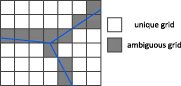
Unique cell and ambiguous cell
-
Ambiguous grid. A grid cell g is an ambiguous cell if there exist two different points p t 1≠p t 2 in g, such that NF(pt 1)≠NF(pt 2).

The following theorem provides a method to classify a cell being unique or ambiguous.
Theorem 1.
Let p t i (i=1,2,3,4) be grid g’s four vertices. If there exists a facility f such that for all points pt in g, N F(p t)=f, then g is a unique cell.
Proof.
Assume p t 1 is the farthest vertex from facility f, then for every point pt in g, d(pt,f)≤d(p t 1,f), where d(x,y) is the Euclidean distance. Since N F(p t 1)=f, we can get N F(p t)=f. Hence, g is a unique cell.
Due to the existence of ambiguous cells, we use approximate influence instead of accurate facility influence. For every facility f in \(\mathcal {F}\), the approximate influence of facility f is defined as follows:
where NF(g) denotes the nearest facility of grid cell g, H(p) outputs the cell that p is mapped to, and Pr(·) is the probability.
Since every object can be mapped to a cell, we separate the objects set \(\mathcal {P}\) into two subsets: one is unique cell set \(\mathcal {P'}\) and the other is ambiguous cell set \(\mathcal {P''}\). If the mapped cell g is a unique cell, then Pr(NF(g)=f|g=H(p))=1; when the mapped cell g is an ambiguous cell, we design three methods to compute Pr(NF(g)=f|g=H(p)).
Case 1 (Centering): When object p is mapped to grid g, we use the center of g (denoted by c) representing grid g to compute the probability.
Case 2 (Sampling): We randomly choose several points in a grid and thus compute every sampling point’s nearest facility in \(\mathcal {F}\). The sampling points are uniformly distributed.
where s is a sampling point and \(\mathcal {S}_{g}\) is the set of sampling points.
Case 3 (Area): We partition a grid using the Voronoi diagram, then we compute the area of each part and use the proportion related to facility f as the probability. Suppose all points in R 1 are in f, then
Centering is the simplest scheme as it uses center point to represent a grid and finding the nearest facility of a point is easy. However, it is too coarse-grained because it increases the inaccuracy if one object does not lie in the same region as the center. If locations mapped to a grid follow uniform distribution, sampling and area schemes are recommended. The area scheme is a generalization of the sampling scheme and can use the information of Voronoi diagram [19] generated by facility set \(\mathcal {F}\).
A natural question now arises: what is the difference between a facility’s actual influence and approximate influence? If we assume objects follow uniform distribution, then we have the following theorem.
Theorem 2.
Given a region R, facility set \(\mathcal {F}\), object set \(\mathcal {P}\), and a grid partition with grid size l, for a facility \(f \in \mathcal {F}\), we have
Proof.
Set \(\mathcal {P}\)consists of two subsets: a unique cell set \(\mathcal {P'}\) and an ambiguous cell set \(\mathcal {P''}\). When l gets smaller, the number of objects in \(\mathcal {P'}\) decreases and thus the ambiguity of influence of facility f will decrease. Therefore, there exits a small l ∗, such that for all l<l ∗, \(\mathcal {P''}=\Phi \). Thus, we have
Theorem 2 shows that if l is small, the approximate influence of a facility is very close to its actual influence. We can use \(\hat I_{\mathcal {P}}(\,f)\) to approximately estimate \(I_{\mathcal {P}}(\,f)\) if the grid size is not too big. In practical, we also shall not set the grid size too small. We demonstrate the reason below.
3.3 Grid size
Grid size l has an impact to facility influence on three aspects: memory size requirements, computing overhead, and accuracy. We next analyze these three factors and discuss how to determine a suitable grid size.
Memory Intuitively, smaller grid size makes a larger grid count in a certain geographic region. For instance, assume Beijing has an area of S (nearly to 16,800 km2), the grid count is equal to S/l 2 where l is the grid length. If one grid only stores one value, i.e., facility influence (assume 32-bit), then the total memory needed is equal to (S/l 2)∗32 bits. We generally do not set grid size too small considering memory usage.
Computing overhead. Given N facilities and M objects, each object p falls into one grid, so overhead of computing facility influence is Θ(1) for this object-facility pair. The total computing overhead is Θ(M), which is irrelative with grid size.
Accuracy If we set l larger, we have fewer unique cells and more ambiguous cells, which will decrease the accuracy of facility influence. The principle is not to set l too large. Empirically, we set l to be average distance of adjacent facilities. In the evaluation section, we would discuss the grid size impacting over facility influence.
3.4 Facility influence computation
After the entire geographic region is divided into cells, we can get a mapping between cells and facilities. Given an object’s location, the grid index indicates which cell the object should be mapped. The corresponding nearest facility and its probability can be retrieved. Therefore, it is unnecessary to compute distance between all facilities and the object to determine the nearest facility. Our iterative process works as shown in Algorithm 1. When an object’s location is updated (i.e., changed), we use grid index to get a new grid cell ID. If the current cell ID is not equal to the previous one, we extract the new nearest facility ID which is stored in the grid data structure. We then compare the current facility ID with the previous one. If they are equal, we just skip and do nothing. Otherwise, we plus facility influence value into current facility and minus it from the previous one. Then, we calculate the facility influence using (3).

Analysis: The time complexity of Algorithm 1 is O(N), where N is the number of objects. Lines 2 and 3 describe that the grid cell ID is obtained from object’s location using grid index, so the calculation is constant time. Lines 5 and 6 retrieve data from grid data structure, which also takes constant time. The upper bound of algorithm is determined by the the number of objects.
4 Influence prediction
The influence of a facility is determined by the number of vehicles gathered around it. Intuitively, vehicles have their trajectories and their future locations can be predicted from their historical movement patterns. First-order Markov chain model (MM) can be used to estimate the probability of a vehicle’s next location, but it suffers from weak predictive ability. In addition, it is hard to learn a high-order Markov model due to the data sparsity problem. In this section, we present how to use TMM to predict objects’ location in the future based on their trajectories. Specifically, we first discuss how to construct a Markov model, then present the details of TMM. Finally, we propose an algorithm that predicts a facility’s future influence under TMM.
4.1 Construction of Markov model
We have previously used a grid partition-based approach to calculate facility influence. Now, we utilize the same grid representation as in the previous section to predict a vehicle’s future location. Partitioned grids can be converted to a grid graph, where each node is one grid and an edge exists between two nodes implying that the two grids are adjacent.
There are two advantages using a grid partition-based approach. First, a grid representation is appropriate for facility influence prediction. Second, a grid-based approach can avoid the data sparsity problem when predicting future location. When a trajectory consists of a sequence of locations, it can be represented using a sequence of grids. Therefore, we will have lots of trajectory data in grid index to represent each trajectory. For predicting future locations with historical trajectories, lots of training data is needed for our TMM model.
Each grid cell is viewed as a state and the Markov model uses these states to build its state transition matrix. In the matrix, the transition probability between grid cells (i.e., states) is trained by the historical step counts, i.e., the number of transition steps from one cell to another is used to derive the transition probability between these two cells. To further understand the processing of Markov model for trajectories, we use an example to illustrate it. In Fig. 4, the region is partitioned into 3×3 grids. Trajectory T 1 is a sequence of grid cells: g 1,g 4,g 5 (Fig. 4 a). Each grid is a state in Markov model, so T 1 is represented as a sequence of states over time (Fig. 4 b).

An example of using Markov model. a grid partition for trajectory. b 3×3 Markov model for trajectory
The prediction of objects’ future locations consists of two phases: a training phase where the historical trajectories are mined offline to obtain transition matrix and an online prediction phase where the historical trajectory of a given object is analyzed and its future locations are predicted.
In the training phase, a Markov model is established by associating a state with each grid g i . Two directed transitions of states corresponding to adjacent grids g i and g j are established, i.e., g i to g j and g j to g i . Let S ij denotes a travel from g i to g j . The transition probability of S ij is denoted by P r(S ij ). Note that a trajectory T ij is composed of a set of steps: T ij ={S i,i+1,S i+1,i+2,⋯,S i+n, j }. Formally,
where |S i¬| is the total number of travels from g i to all neighboring cells.
For each pair of adjacent nodes in the grid graph, we compute the transition probabilities offline using Eq. (4). These probabilities are stored as entries of a two-dimensional matrix where one dimension corresponds to the node of current state and the other dimension corresponds to the next state. We denote the matrix and its entries by the transition matrix M and M ij , respectively.
4.2 Prediction of future locations
Prediction of object’s future locations essentially provides a set of cells that the object will reside along with a probability. We next use an example (Fig. 5) to illustrate how to predict future location using TMM model. Suppose one object p currently stays at grid cell g 5. Next time, it has four possible movements: g 2, g 4, g 6, and g 8 (Fig. 5 a). If its trajectory is unknown, the transition probability (in the transition probability matrix of Markov model) is directly used as the probability of it going to each of the four cells. If its trajectory is known, we can use Bayesian theorem to calculate the probabilities (Fig. 5 b), where prior probability is the transition probability and the likelihood probability is how the trajectory and the historical data is similar to each other.

Trajectory-based Markov model. a Normal transition. b Transition based on trajectory
We then formulate the prediction with objects trajectory based on TMM. Assume one object is currently in cell g j with trajectory T ij , i.e., it has gone through a certain path from g i to g j . Now the question is how to derive the probability of the object arriving at an adjacent cell g k in the next time unit, given the knowledge of T ij ? This probability can be computed using Bayes rule as follows.
where P r(S jk )=P r jk can be obtained from transition matrix M. P r(T ij |S jk ) denotes the probability of an object traveling from g i to g j given that transition steps are from grid j to grid k. It can be computed as follows [20].
where P r i→k is the total transition probability of all possible trajectories traveling from g i to g k . Combining Eq. (6) and Eq. (5), we have
P r(S jk ) can be obtained from transition matrix M. In fact, P r i→k can also be calculated from M. In general, M r(r∈[0,∞)) holds the probabilities of transition from one node to another in exactly r steps (i.e., M r holds r-step transition probabilities). One method [20] to compute P r i→k is
where L i→k denotes l 1 distance (step count of the shortest path) from g i to g k and L de,i→k denotes the maximal steps where an object may run more paths from g i to g k . L de,i→k is often set to be 0.2L i→k .
4.3 Prediction of future facility influence
Facility influence is determined by objects around them. If we can predict these objects’ future locations, then we can predict facility influences in the future. This raises several interesting challenges. One challenge is how to select a proper time step size. Objects have different speed and direction, e.g., taking a taxi requires a larger time step size compared with walking. Mobility is also affected by surrounding environments, such as traffic congestion or speed limitation. It is hard to predict when objects will arrive at the predicted place even though we make a successfully prediction. The other challenge is that the prediction is related to the size of grid cell. If the cell is too small, object may cross several cells in one time step, resulting in data sparsity problem for the training phase of the Markov model construction; if the cell is too large, object will stay in one cell for several time steps, resulting in inaccuracy to facility influence. In our experiments, we have tried multiple cell size from 100 to 1000 m and empirically selected an appropriate value.
The speed of an object is related to the object’s previous speed. If we can get these two pieces of information as well as the speed, we can determine the grid cells the object will arrive. To be specific, suppose travel time is t, the speed is v, so the distance from current location is s=v t. Then, we can get a set of possible cells C within distance s from current location. If cell g in C is next to current cell, we can directly use Eq. (7) to compute the probability. After getting all possible cells’ probability, we can use the highest one as the final prediction result for that object. Algorithm 2 summarizes how prediction of facility influence is done.

5 Performance evaluation
Our evaluation consists of three parts: (1) memory usage and computing overhead for grid partition and indexing, (2) overhead and accuracy of facility influence computing, and (3) prediction accuracy of facility influence prediction.
5.1 Experimental methodology
To validate the effectiveness and efficiency of proposed algorithms, we take taxis as moving objects for facility influence computation. We use a large real-world dataset which consists of 1-month moving trajectories of taxis in Beijing. It contains more than 27,000 taxis over one billion trajectories. Facilities are overpasses, subway stations, tourism destinations, shopping malls, etc, which are extracted from over 1000 Beijing POIs [7]. Each taxi uploaded its location to the database server every 30 s. Figure 6 a shows the coverage of taxis in 1 day. We can see that taxi trajectories almost cover all central urban area of Beijing. Figure 6 b is a typical taxi’s trajectory in a day.

Distribution of taxi trajectories. a Trajectory coverage. b A taxi’s trajectory 1 day
We ran our proposed algorithm on a desktop machine with Intel Core I5-3380 2.90GHz dual core CPU. The data is stored in SQL server database. There are many data structures to construct grid index, such as hash table, hash array, or matrix. We use hash array to index the grids. Each grid use 100 bits to store two values: facility IDs and the corresponding influence value. We train our trajectory-based Markov model with built-in toolkit [21]. We first separate every taxi trajectory into sub-trajectories which starts in one grid cell and ends in another. Then, we split the sub-trajectory database to two parts, one for training Markov transition matrix and the other for testing the effectiveness of our algorithm. We then compute and save the Markov transition matrix M using Eq. (4). It takes several hours to train matrix M using the massive trajectories. We then compute M 2,M 3,⋯ and save them on a hard disk. When doing online prediction, we put all the matrices into memory, avoiding slow matrix multiplication operations.
For evaluation of computing overhead, we use response time to measure the efficiency of our algorithms, which includes CPU time and I/O latency. For evaluating accuracy, we compute two type of positive cases: correct influence calculation ratio and correct influence prediction ratio. Table 1 lists all parameters used in our experiments.
5.2 Grid partition
We first measure memory usage and overhead of grid partition. The memory usage is on the grid index. Table 2 lists memory usage of grid index with various grid sizes, increasing from 10 to 1000 m; 10 m is close to GPS location precision. The larger grid size, the more memory space in a fixed geographic region. In our experiments, Beijing has an area size of 16,800 km2, with the smallest grid size of 10 m (GPS precision is close to 10 meters), we need 2.5 GB memory. This is acceptable in our case.
Figure 7 depicts the running time to different grid partitions. The running time increases along with the increase in the number of facilities from 100 to 500, in Fig. 7 a. This is because grid partition needs to calculate every facility’s scope and then map it into grid cells, larger facility count leads to higher computing overhead. Figure 7 b depicts the impact of grid size on running time. It confirms our intuition that smaller grid size causes higher computing overhead in grid partition. The smaller the grid size, the higher the grid count in a fixed geographic region.

Computing overhead of grid partition. a Impact of facility count on overhead in grid partition. b Impact of grid size on overhead in grid partition
In brief, if grid size l is too small, the index requires larger memory space and higher overhead. We propose to set l from 100 to 500. The facility count depends on specific application scene, which affects the computing overhead.
5.3 Facility influence computing
We evaluate Algorithm 1 for calculating the facility influence. Figure 8 a depicts how taxi count affects the response time of facility influence calculation. In these experiments, we set grid size l=100 and facility count m=300. The calculation only takes 100 ms when the taxi count is close to 10,000. The response time increases very slowly with the increase of taxi count n. This is because the calculation maps location to grid index, which has a constant complexity Θ(1). Figure 8 b shows how facility count affects response time. In these experiments, grid size is l=100 and taxi count n=10,000. Our approach remains very efficient and the response time is under 0.5 s. These results have confirmed that using grid is suitable for calculating facility influence in real time.

Overhead of calculating facility influence. a Impact of taxi count on overhead of facility influence calculation. b Impact of facility count on overhead of facility influence calculation
We next evaluate the effectiveness of dealing with ambiguous grids. We basically measure the accuracy of associating objects with facility. We consider the ground truth being the closest facility in Euclidean distance. In these experiments, facility count m=300 and taxi count n=10,000. Figure 9 depicts the results using the three methods we proposed: centering (a), sampling (b), and area (c). If grid size is too large, there are large ambiguous grids at the intersection of multiple facilities. The accuracy decreases with the increase of grid size. When the grid length becomes 1000 m, the accuracy of all three methods is unacceptable with the worst case close to 56 %. When the grid size is small (i.e., close to 100 meters), the accuracy of all three methods stays high (i.e., close to 96 %.) Combining the results of grid partition shown in Fig. 7 and Table 2, large grid size indicates low memory usage and low overhead. We suggest to set l between 100 and 500 m according to different surroundings (various facility types). Fig. 9 also depicts the accuracy with different k values, i.e., calculating top k most influential facilities. If k equals facility count m, it basically calculates influence for all facilities. Here, we measure different k values impacting facility influence calculation (total count is 300), including 10, 50, 80, and 100. There is no difference in accuracy regardless of the k value.

Accuracy of associating objects with facility. a Centering. b Sampling. c Area
5.4 Prediction accuracy
We firstly evaluate location prediction accuracy of our TMM. Two factors affect the accuracy: the trajectory length and the number of steps taken. Step indicates that the location is transformed from one grid cell to another cell (includes jumping circle). Figure 10 depicts the impact of trajectory length on location prediction accuracy (assume future step is 1). When the trajectory length is long (10 steps in this case), the accuracy is close to 85 %. When the number of historical steps equals 1, the accuracy is below 70 %. This is reasonable since more historical data will lead to higher accuracy in prediction. The cumulative distribution function (CDF), as shown Fig. 10 b, depicts that the accuracy is higher than 80 % on average.

Prediction accuracy with trajectory length. a Historical step count. b CDF under historical steps
In order to verify the effectiveness of our TMM for future step count, we compare it with the naive MM which is considered as baseline. MM is a common methods in location prediction with normal transition, which directly uses the transition probability of current state to neighbors. The trajectory length used for TMM and MM ranges from 3 to 10.
Figure 11 a depicts impact of future steps on the prediction accuracy. The accuracy of TMM is much higher than MM in every steps, which indicates that historical trajectories can to a large extent dominate future locations. Figure 11 b shows the CDF of prediction accuracy of the two models: for 80 % of the time, the prediction accuracy in TMM is lower than 80 %. While the prediction accuracy in MM is lower than 40 %, which is significantly lower than TMM.

Prediction accuracy with future step count. a Future step count. b CDF under future steps
For the trajectory length, we suggest to use a longer one so that the prediction accuracy is higher. For large future step count, the prediction accuracy seems low from our experiments. However, it does not affect the facility influence prediction. This is because when the taxi is moving within the scope of a facility, prediction error in future location cannot cause the error in facility influence prediction. The error in influence prediction only occurs when the taxi moves from the scope of one facility to another, which case error occasionally occurs in future step prediction.
We next evaluate the effectiveness of predicting facility influence. We set the parameters l=500,m=500,n=30,000; the historical steps is bigger than 4 and we only consider the situation in 5 future steps. The ground-truth of our test uses nearest distance to calculate the facility influence. We use the sampling method to deal with ambiguous grids. Figure 12 a depicts the accuracy of dealing with ambiguous grids and also future influence prediction. We can see that our facility influence prediction accuracy is close to the accuracy of location prediction, i.e., above 80 % in all k values tested. Our facility influence calculation accuracy has better accuracy than prediction by nearly more than 10 %, and this difference is caused by the error in future location prediction. Figure 12 b shows the CDF of facility influence prediction accuracy. Our solution has achieved an acceptable accuracy for predicting facility influence.

Accuracy of facility influence prediction. a Accuracy of prediction and computing. b CDF under prediction
We observe that although location prediction can introduce uncertainty which then affects the final influence prediction, as long as the predicted grid is not far away from the real location and they have the same nearest facility, this uncertainty has weak impact on influence prediction.
6 Related work
Our work lies at the intersection of urban computing and facility influence query in databases.
Urban computing. Urban computing is emerging as a concept where every sensor, device, person, vehicle, building, street, and so on in urban areas can be used as a component to probe city dynamics and further enable a city-wide computing for serving people and their cities. Previous work has mainly focused on solving specific issues that urban residents face, such as measuring air pollution of POIs using human mobility in different city regions [7], recommending taxi routes [22, 23], or inferring energy consumption of city via the car refueling behavior [24]. These works mostly focus on dynamic locations due to human mobility, but less on facility influence.
Cyber-physical vehicles. In general, cyber-physical vehicles are equipped with vehicular cyber-physical systems in which various vehicles are networked to sense, monitor, control, and communicate with the physical world. Cyber-physical vehicles have attracted significant attention recently [25]. Different from the existing work on cyber-physical systems, recent studies on cyber-physical vehicles focus on message dissemination optimization [26], traffic volume measurement [27], data dissemination [28], integrating with mobile cloud computing [29], and so on. Our work use cyber-physical vehicles (typically considered as dynamic objects in urban computing) to research the changes in influence of facility (usually focus on static facility in the databases community). The increasing availability of GPS-embedded cyber-physical systems provides large scale taxi trajectories in urban computing. Many works have studied taxi trajectories and then proposed strategies for improving taxi drivers’ income by analyzing the pick-up and drop-off behavior of taxicabs in different locations [30, 31]. We also use taxi trajectories; however, we use them to consider how vehicles impact facility influence.
Facility influence. In the database community, facility influence calculation is mainly focused on spatial query processing over different geographic regions. Korn and Muthukrishnan [9] propose reverse nearest neighbor as influence indicator to measure top k most influencial web sets. Other work [10, 11, 32] extends web set queries to the spatial place in geographic region. These previous works usually construct two R-tree structures in memory, in which objects are stationary, but writing to and reading from the database to load the memory is major cost. Different from these existing works, our work focuses on the dynamic objects in a geographic area. Several previous works [19, 33] propose the preprocessing stage to efficiently compute rather than using R-tree. Voronoi-based partition [19] divides scopes of facility into various region-irregular areas, and each area represents the scope of a facility. This approach requires to build tree index for Voronoi partition and time cost over query Voronoi index is related to area count. Reference [33] adopts adaptive grid partition to find influential locations. Similar to Voronoi-based partition, adaptive grid also requires R-tree indices to identify right grid number to calculate the facility influence. In contrast, our work adopts grid partition with uniform grids. Regular area partition can be indexed with a simple data structure, so its query time is constant.
7 Conclusions
In this paper, we propose to predict the influence of a facility in smart city, under large-scale dynamic cyber-physical vehicles. A facility supports public services to satisfy the needs of people’s urban lives, and its influence is affected by the count of vehicles gathered around it. We present a grid partition approach to efficiently compute facility influence over dynamic vehicles. To predict facility influence in the future, TMM model trained by historical trajectories is proposed to predict vehicle’s future movement, which is then used to evaluate future influence of facilities. Experimental results show that our approaches are acceptable in terms of both computing facility influence in real time and predicting future facility influence with high accuracy.
References
M Lukasiewycz, S Steinhorst, F Sagstetter, W Chang, P Waszecki, M Kauer, S Chakraborty, in 15th Euromicro Conference on Digital System Design, DSD 2012. Cyber-physical systems design for electric vehicles (Cesme, IzmirTurkey, 2012), pp. 477–484.
DPF Möller, T Deriyenko, H Vakilzadian, in IEEE International Conference on Electro/Information Technology, EIT 2015. Cyber-physical vehicle tracking system: Requirements for using a radio frequency identification technique (Dekalb, ILUSA, 2015), pp. 552–557.
T Kindberg, M Chalmers, E Paulos, Guest editors’ introduction: Urban computing. Pervasive Comput. IEEE. 6(3), 18–20 (2007).
Y Zheng, L Capra, O Wolfson, H Yang, Urban computing: Concepts, methodologies, and applications. ACM Transaction on Intelligent Systems and Technology. 5(3), 222–235 (2014).
Y Zheng, Y Liu, J Yuan, X Xie, in UbiComp 2011: Ubiquitous Computing, 13th International Conference. Urban computing with taxicabs (UbiComp 2011Beijing, China, 2011), pp. 89–98.
S Chawla, Y Zheng, J Hu, in 12th IEEE International Conference on Data Mining, ICDM 2012. Inferring the root cause in road traffic anomalies (BrusselsBelgium, 2012), pp. 141–150.
J Yuan, Y Zheng, X Xie, in The 18th ACM SIGKDD International Conference on Knowledge Discovery and Data Mining, KDD ’12. Discovering regions of different functions in a city using human mobility and POIs (ACMBeijing, China, 2012), pp. 186–194.
L Wei, W Peng, W Lee, Exploring pattern-aware travel routes for trajectory search. ACM TIST. 4(3), 48 (2013).
F Korn, S Muthukrishnan, in Proceedings of the 2000 ACM SIGMOD International Conference on Management of Data. Influence sets based on reverse nearest neighbor queries (Dallas, Texas, USA., 2000), pp. 201–212.
J Huang, Z Wen, J Qi, R Zhang, J Chen, Z He, in Proceedings of the 20th ACM Conference on Information and Knowledge Management, CIKM 2011. Top-k most influential locations selection (Glasgow, United Kingdom, 2011), pp. 2377–2380.
T Xia, D Zhang, E Kanoulas, Y Du, in Proceedings of the 31st International Conference on Very Large Data Bases. On computing top-t most influential spatial sites (Trondheim, Norway, 2005), pp. 946–957.
J Gao, J Li, Z Cai, H Gao, in 2015 IEEE Conference on Computer Communications, INFOCOM 2015. Composite event coverage in wireless sensor networks with heterogeneous sensors (KowloonHong Kong, 2015), pp. 217–225.
Z Cai, Z Chen, G Lin, A 3.4713-approximation algorithm for the capacitated multicast tree routing problem. Theor. Comput. Sci. 410(52), 5415–5424 (2009).
Z Cai, G Lin, G Xue, in Computing and Combinatorics, 11th Annual International Conference, COCOON 2005. Improved approximation algorithms for the capacitated multicast routing problem (KunmingChina, 2005), pp. 136–145.
Z He, Z Cai, S Cheng, X Wang, Approximate aggregation for tracking quantiles and range countings in wireless sensor networks. Theor. Comput. Sci. 607:, 381–390 (2015).
J Li, S Cheng, H Gao, Z Cai, Approximate physical world reconstruction algorithms in sensor networks. IEEE Trans. Parallel Distrib. Syst. 25(12), 3099–3110 (2014).
S Cheng, Z Cai, J Li, X Fang, in 2015 IEEE Conference on Computer Communications, INFOCOM 2015. Drawing dominant dataset from big sensory data in wireless sensor networks (KowloonHong Kong, 2015), pp. 531–539.
L Zhan, Y Zhang, W Zhang, X Lin, in 21st ACM International Conference on Information and Knowledge Management, CIKM’12. Finding top k most influential spatial facilities over uncertain objects (Maui, HIUSA, 2012), pp. 922–931.
P Zhang, R Cheng, N Mamoulis, M Renz, A Züfle, Y Tang, T Emrich, in 29th IEEE International Conference on Data Engineering, ICDE 2013. Voronoi-based nearest neighbor search for multi-dimensional uncertain databases (BrisbaneAustralia, 2013), pp. 158–169.
AY Xue, R Zhang, Y Zheng, X Xie, J Huang, Z Xu, in 29th IEEE International Conference on Data Engineering, ICDE, 2013. Destination prediction by sub-trajectory synthesis and privacy protection against such prediction (BrisbaneAustralia, 2013), pp. 254–265.
Hidden Markov Model (HMM) Toolbox. https://www.cs.ubc.ca/~murphyk/Software/HMM/hmm.html.
L-Y Wei, Y Zheng, W-C Peng, in The 18th ACM SIGKDD International Conference on Knowledge Discovery and Data Mining, KDD ’12. Constructing popular routes from uncertain trajectories (BeijingChina, 2012), pp. 195–203.
A Bassoli, J Brewer, K Martin, P Dourish, S Mainwaring, Underground aesthetics: Rethinking urban computing. Pervasive Comput. IEEE. 6(3), 39–45 (2007).
F Zhang, D Wilkie, Y Zheng, X Xie, in The 2013 ACM International Joint Conference on Pervasive and Ubiquitous Computing, UbiComp ’13, Zurich. Sensing the pulse of urban refueling behavior (ACMZurich, Switzerland, 2013), pp. 13–22.
D Jia, K Lu, J Wang, X Zhang, X Shen, A survey on platoon-based vehicular cyber-physical systems. IEEE Commun. Surv. Tutor. 18(1), 263–284 (2016).
H Zheng, J Wu, in 35th IEEE International Conference on Distributed Computing Systems, ICDCS 2015. Optimizing roadside advertisement dissemination in vehicular cyber-physical systems (Columbus, OHUSA, 2015), pp. 41–50.
Y Zhou, S Chen, Z Mo, Q Xiao, in 35th IEEE International Conference on Distributed Computing Systems, ICDCS 2015. Point-to-point traffic volume measurement through variable-length bit array masking in vehicular cyber-physical systems (Columbus, OHUSA, 2015), pp. 51–60.
K Liu, VCS Lee, JK Ng, J Chen, SH Son, Temporal data dissemination in vehicular cyber-physical systems. IEEE Trans. Intell. Trans. Syst. 15(6), 2419–2431 (2014).
J Wan, D Zhang, Y Sun, K Lin, C Zou, H Cai, VCMIA: A novel architecture for integrating vehicular cyber-physical systems and mobile cloud computing. MONET. 19(2), 153–160 (2014).
Y Ge, C Liu, H Xiong, J Chen, in Proceedings of the 17th ACM SIGKDD International Conference on Knowledge Discovery and Data Mining. A taxi business intelligence system (ACMSan Diego, CA, USA, 2011), pp. 735–738.
J Yuan, Y Zheng, L Zhang, X Xie, G Sun, in UbiComp 2011: Ubiquitous Computing, 13th International Conference. Where to find my next passenger (UbiComp 2011Beijing, China, 2011), pp. 109–118.
J Liu, G Yu, H Sun, in Proceedings of the 20th ACM Conference on Information and Knowledge Management, CIKM 2011. Subject-oriented top-k hot region queries in spatial dataset (GlasgowUnited Kingdom, 2011), pp. 2409–2412.
D Yan, RC-W Wong, W Ng, in Proceedings of the 20th ACM Conference on Information and Knowledge Management, CIKM 2011. Efficient methods for finding influential locations with adaptive grids (Glasgow, United Kingdom, 2011), pp. 1475–1484.
Acknowledgements
This work was supported by the National Natural Science Foundation of China (Grant No.61402463), the “Strategic Priority Research Program” of the Chinese Academy of Sciences (Grant No.XDA06040101), and the Young Talent Program of Institute of Information Engineering Chinese Academy of Sciences (Grant No.1102008202).
Author information
Authors and Affiliations
Corresponding author
Additional information
Competing interests
The authors declare that they have no competing interests.
Rights and permissions
Open Access This article is distributed under the terms of the Creative Commons Attribution 4.0 International License (http://creativecommons.org/licenses/by/4.0/), which permits unrestricted use, distribution, and reproduction in any medium, provided you give appropriate credit to the original author(s) and the source, provide a link to the Creative Commons license, and indicate if changes were made.
About this article

Cite this article
Wang, H., Li, Q., Yi, F. et al. Influential spatial facility prediction over large scale cyber-physical vehicles in smart city. J Wireless Com Network 2016, 103 (2016). https://doi.org/10.1186/s13638-016-0606-4
Received:
Accepted:
Published:
DOI: https://doi.org/10.1186/s13638-016-0606-4